Unlocking the Potential of PRISMA Hyperspectral Imagery for Precision Agriculture Mapping
Background
This project evaluates the effectiveness of PRISMA hyperspectral imagery for leaf area index (LAI) estimation and vegetation trait mapping. By integrating PROSAIL radiative transfer simulations, ground-truth LAI measurements, and machine-learning regression models, we benchmark accuracy, robustness, and spatial consistency across multiple experimental configurations.
The Leaf Area Index (LAI) is a critical indicator for understanding vegetation health, ecosystem monitoring, and precision agriculture. However, current methods for detecting LAI face challenges such as sensitivity to environmental variations and inaccuracies in modeling approaches. Hyperspectral remote sensing data provides a solution by capturing detailed spectral information, enabling the analysis of key biophysical traits such as chlorophyll and water content. Our study addresses these challenges by developing an integrated approach that combines PROSAIL modeling, sensitivity analysis to improve LAI detection accuracy and vegetation mapping.
Objective: Design a robust, reproducible pipeline that improves LAI prediction accuracy while remaining operationally scalable.
Methodology Overview
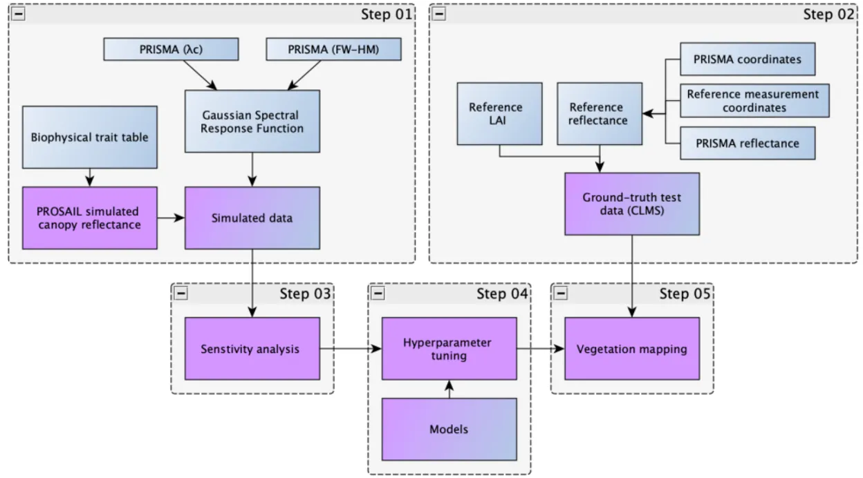
The workflow consists of five tightly-coupled stages:
Step 01 — PROSAIL Simulation
| Description | Units | Parameter | Min | Max |
|---|---|---|---|---|
| Chlorophyll a + b content | ug/cm2 | Cab | 5 | 90 |
| Equivalent water thickness | cm | Cw | 0.003 | 0.03 |
| Leaf area index | – | LAI | 0.01 | 8 |
| Leaf structure index | – | N | 1 | 3.5 |
| Carotenoid concentration | ug/cm2 | Car | 1 | 20 |
| Brown pigment | – | Cbrown | 0 | 1 |
| Dry matter content | g/cm2 | Cm | 0.002 | 0.01 |
| Average leaf angle (Ellipsoidal distribution) | – | LIDFa | 0 | 90 |
| Dry/Wet soil factor | – | ρsoil | 0.5 | 1.5 |
| Soil brightness factor | – | αsoil | 0 | 1 |
| Hotspot parameter | – | hspot | 0 | 3.5 |
| Solar zenith angle | deg | tts | 0 | 70 |
| Observer zenith angle | deg | tto | 0 | 90 |
| Relative azimuth angle | deg | phi | 0 | 90 |
We initiated the simulation process by defining a biophysical traits table. Unlike fixing the traits, our approach allows for a broader exploration of parameter space, which is crucial for capturing real-world variations in vegetation. This ensures that the simulated reflectance closely aligns with the complexities of natural vegetation. Importantly, we maintain uniform parameter distributions and random concatenation across the desired size to avoid introducing artificial biases. This approach guarantees that our simulations accurately represent the range of real-world scenarios.
We used a common radiative transfer model named PROSAIL to stimulate the process.
- Generated PRISMA-like hyperspectral reflectance using the PROSAIL RTM.
- Simulated variability across LAI, chlorophyll content (Cab), and water thickness (Cw).
- Provided a controlled baseline for sensitivity testing and model training.
Step 02 — Ground-Truth Preprocessing
To ensure the accuracy of our study, we collected trustworthy LAI (Leaf Area Index) data from 29 locations as part of the Ground-Based Observations for validation program through the Copernicus Land Monitoring Service. These measurements were taken between December 2020 and May 2022.
We carefully selected data by removing entries without precise coordinates, ensuring exact location accuracy. Matched with PRISMA L2D scenes using:
- ±3-day temporal window
- ≤15% cloud cover
- Reflectance normalization (zero bands removed for consistency)
A high-quality subset of 50 test samples from 8 sites shown below was reserved for validation.
| Site | Land Cover Type | Reference Measurements | PRISMA Images Acquired |
|---|---|---|---|
| Bartlett Experimental Forest | Mixed Forest | 5 | 1 |
| Guanica Forest | Evergreen Broadleaf | 3 | 1 |
| Harvard Forest | Mixed Forest | 5 | 2 |
| Oak Ridge | Mixed Forest | 3 | 1 |
| Ordway Swisher Biological Station | Evergreen Needleleaf | 8–2 | 3 |
| Smithsonian Conservation Biology Institute | Mixed Forest | 2–1 | 2 |
| Talladega National Forest | Evergreen Needleleaf | 11 | 4 |
| Underc | Mixed Forest | 7–1 | 3 |
Step 03 — Sensitivity Analysis
- Evaluated spectral sensitivity of LAI across 400–2500 nm.
- Assessed interactions between LAI, Cab, and Cw.
- Analysis performed on:
- Simulated PRISMA reflectance
- Ground-truth LAI test data
This step informed band importance and model configuration choices:
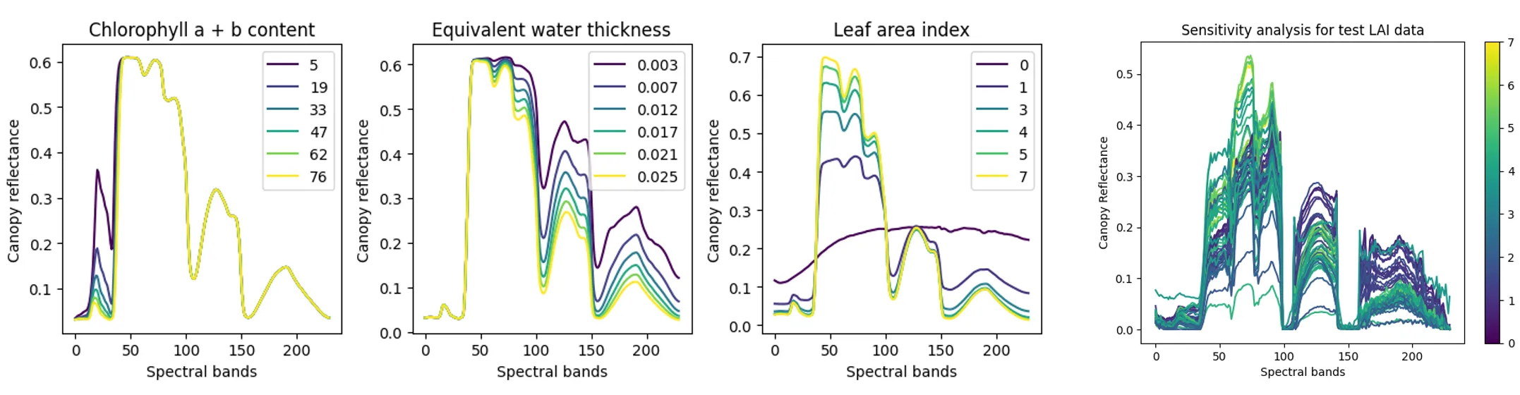
Accordingly to above, Chlorophyll influences the visible spectrum—particularly near the blue (430–450 nm) and red (640–680 nm) bands due to chlorophyll absorption. Water thickness affects reflectance in the 100–150 spectral band, linked to water absorption in the shortwave infrared. LAI impacts reflectance across the full spectrum, especially as canopy density increases.
To validate the simulation, we compared this against ground-truth test data (graph on the top right). This step was crucial to identify sensitive bands and confirm that simulated reflectance aligns with real-world observations—setting the stage for our model training and mapping work.
Step 04 — Hyperparameter Tuning
- Models evaluated:
- Random Forest (RF)
- Artificial Neural Network (ANN)
- Gaussian Process Regression (GPR)
Training conducted on datasets of varying sizes including 50 / 100 / 200 / 500 samples. Each dataset underwent 50 initialization cycles with 5-fold cross-validation. R-squared measures how well the model’s predictions align with actual observations, indicating goodness of fit; higher scores signify better performance.
Objective: ensure fair comparison and prevent overfitting under limited data regimes.
| Model | Hyperparameter | Values Tested |
|---|---|---|
| Multilayer Perceptron (MLP) | Hidden layer sizes | 64, 128, 256 (single-layer); combinations for multi-layer |
| Activation functions | ReLU, Tanh | |
| Initial learning rate | 0.01, 0.001 | |
| Maximum iterations | 50, 100, 500 | |
| Gaussian Process Regressor (GPR) | Kernel | Matern, RBF, Rational Quadratic |
| Target normalization | True, False | |
| Random Forest Regressor (RDF) | Max depth | None, 10, 50, 100, 500 |
| Number of estimators | 10, 50, 100 |
Building on these insights, we systematically tested combinations of hyperparameters within a predefined search space to identify the optimal settings for each model. The explored hyperparameter space for different models are demonstrated in the table above.
Step 05 — Vegetation Trait Mapping
To evaluate model robustness and consistency, we defined four experimental configurations based on PROSAIL preprocessing choices: normalized vs. unnormalized inputs and fixed vs. unfixed parameters. This factorial design isolates the effects of parameter flexibility and spectral normalization on predictive performance. Each model was trained and evaluated across all four configurations, enabling a systematic comparison of accuracy, stability, and sensitivity to input conditions.
| Code | Description |
|---|---|
| N-F | Normalized + Fixed parameters |
| N-U | Normalized + Unfixed parameters |
| U-F | Unnormalized + Fixed parameters |
| U-U | Unnormalized + Unfixed parameters |
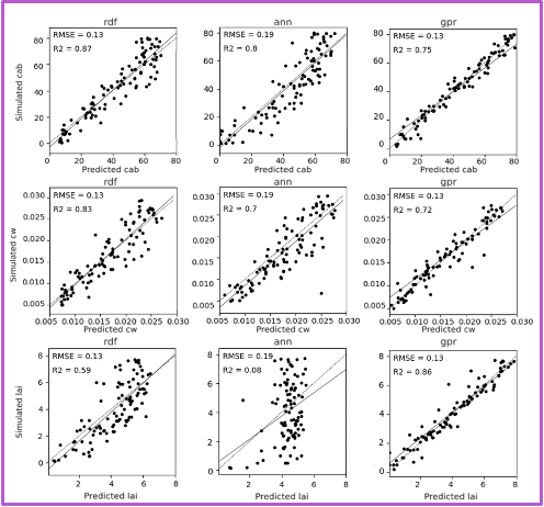
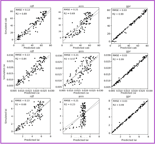

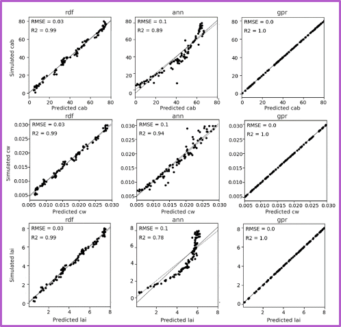
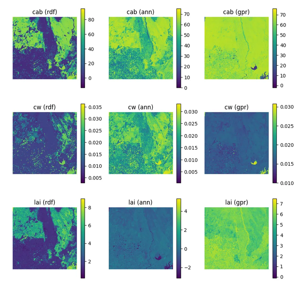
Each row shows predictions for a different biophysical trait—chlorophyll (Cab), water content (Cw), and LAI. Columns in each block shows the performance of three machine learning models. The GPR model, shown in the third column of each block, consistently yields the highest R-squared and lowest RMSE values. The fixed-parameter configurations, particularly when combined with normalized inputs, exhibit tightly clustered predictions along the 1:1 line, reflecting improved stability and reduced variance. In contrast, unfixed configurations, especially under unnormalized conditions, show increased scatter and noise, indicating reduced precision despite greater flexibility.
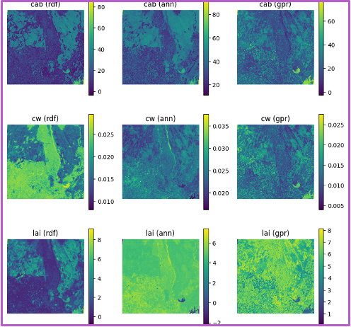
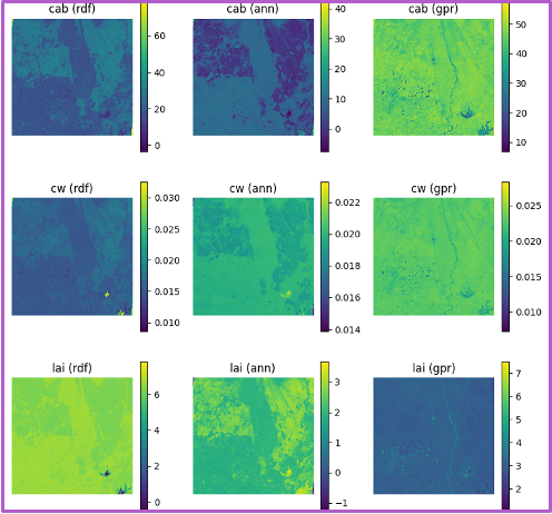
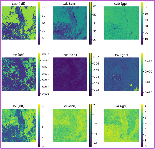
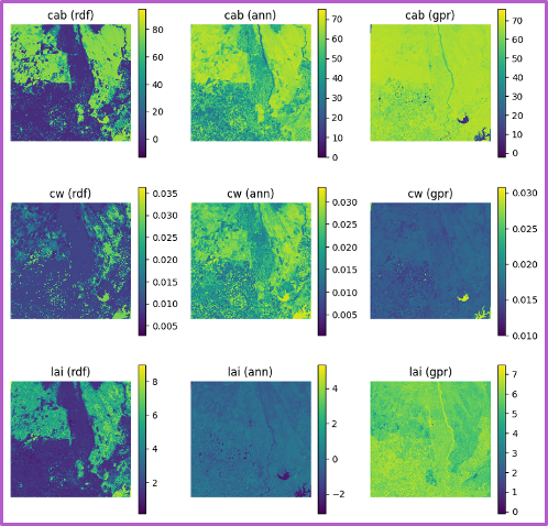
Spatial trait maps reinforce these statistical trends. The normalized–fixed (N-F) configuration produces the most coherent spatial patterns, characterized by smooth gradients, well-defined field boundaries, and minimal artifacts. Conversely, the unnormalized–unfixed (U-U) configuration yields noisier maps with patchy and less interpretable structures. These results highlight a clear tradeoff between model generalization and spatial reliability: while unfixed configurations capture broader variability, fixed and normalized inputs provide more robust and spatially consistent trait estimates, which are critical for downstream applications such as yield modeling, crop monitoring, and early stress detection.
Results
Across all experimental configurations, Gaussian Process Regression (GPR) consistently outperformed both Artificial Neural Networks (ANNs) and Random Forests in prediction accuracy, achieving the highest R² values and lowest RMSE. This indicates that GPR provides estimates that are both precise and reliable across varying input conditions.
The normalized–fixed (N-F) configuration yielded the most stable and consistent results, reflected in both statistical metrics and spatial trait maps. In contrast, unfixed parameter setups introduced greater uncertainty and visible spatial noise, particularly in unnormalized cases, leading to reduced interpretability.
Overall, the PROSAIL–machine learning hybrid framework demonstrates clear improvements in LAI estimation under real-world conditions. Among the evaluated models, GPR emerged as the most effective approach for capturing nonlinear relationships and managing uncertainty in hyperspectral vegetation data.
Key highlights
- Model choice matters: GPR is best suited for hyperspectral LAI retrieval under limited samples.
- Preprocessing is not optional: normalization materially improves robustness.
- Parameter control beats flexibility for operational mapping.
- The proposed pipeline is transferable to other crops and regions with minimal adaptation.
Presented at CSRS 2025 · Lethbridge, Alberta, Canada